Dan Saber

Note: In this post, I assume some familiarity with PyMC. If you need to get up to speed in a hurry and you’re familiar with linear regression, go here for a tutorial. Alternatively, you can read for the methodological intuition, treating the PyMC bits as “readable pseudo-code” that obviate the need for formal mathematical notation.

 Thinking Hierarchically

---

I love looking for new ways to force Bayesian thinking — and, in particular, Bayesian thinking implemented in PyMC — onto my coworkers.

(This is probably one reason they’ve stopped inviting me to parties.*)

A brief example: When dealing with multi-variant experiments in our old A/B testing framework, we would apply Bonferroni corrections to ensure that our analyses retained their Type I Error credibility. In protest, I implemented a utility for building Hierarchical Beta-Binomial Models, and harangued everyone into using it for the purpose of analyzing these simple (albethey multi-variant) tests*^.

(Nobody did, of course, but I got the smug feeling of a job pettily done that defines the discipline of statistics.)

You just said a lot of words. Intuitively, how is your method different from the classical one?

Glad you asked, Bold Italicized Font.

The Beta-Binomial model looks at the success rates of, say, your four variants — A, B, C, and D — and assumes that each of these rates is a draw from a common Beta distribution. Unlike many assumptions (e.g., “Brexit can never happen because we’re all smart and read The New Yorker.“), this one leads to superior inference. In particular, when we assume that all of our success rates come from the same place, we are telling our model to share (or “pool,” to use the parlance) information across variants.

In other words, even when modeling A’s success rate, we may “borrow” information from B, C, and D, depending on how useful we find it. (As we’ll soon see, sample size largely determines usefulness.) Practically speaking, our model will “shrink” our estimate for any given variant’s success rate toward the “grand” estimate, i.e., the success rate of A, B, C, and D combined.

In PyMC2, the model looks like this:

@pymc.stochastic(dtype=np.float64)
def hyperpriors(value=[1.0, 1.0]):
    a, b = value
    if a <= 0 or b <= 0:
        return -np.inf
    else:
        return np.log(np.power((a + b), -2.5))

a = hyperpriors[0]
b = hyperpriors[1]

rates = pymc.Beta('rates', a, b, size=4)

trials = np.array([n] * 4)
successes = np.array(ss)
obs = pymc.Binomial('observed_values', trials, rates,
                    observed=True, value=successes)

mcmc3 = pymc.MCMC([a, b, rates, obs, hyperpriors,
                   trials, successes])

mcmc3.sample(100000, 20000)

And in PyMC3, it looks this:

with pm.Model() as bb_model:

    def ab_likelihood(value):
        a = value[0]
        b = value[1]

        return T.switch(T.or_(T.le(a, 0), T.le(b, 0)),
                        -np.inf,
                        np.log(np.power((a + b), -2.5)))

    ab = pm.DensityDist('ab', ab_likelihood,
                        shape=2, testval=[1.0, 1.0])

    a = ab[0]
    b = ab[1]

    rates = pm.Beta('rates', a, b, shape=4)

    trials = np.array([n] * 4)
    successes = np.array(ss)

    obs = pm.Binomial('observed_values', trials, rates,
                      observed=successes)

For a variant with only a few samples, this shrinkage can reach George Costanzan levels, derailing weekends and ostensibly strong effect sizes alike. Conversely, for a variant with many samples, you might not even be able to distinguish between its shrunken and non-shrunken forms. This, of course, is how it should be: if we can’t make a strong statement about the variant in question, we must look to the others for help — but if we can, we let the variant speak for itself.

(If you come from a Machine Learning or Statistics background, you can think of this as analogous to the regularization parameter in a Lasso or Ridge regression: we avoid overfitting by permitting our inference to be only as strong as the data allows.)

All of this, in turn, grants us the right to make the elegant probabilistic claims which are the hallmark of the Bayesian approach, e.g., “We think there’s a 96% chance B beats C.” No correction needed, even if you proceed to compare B to C then B to A then B to D and so on.

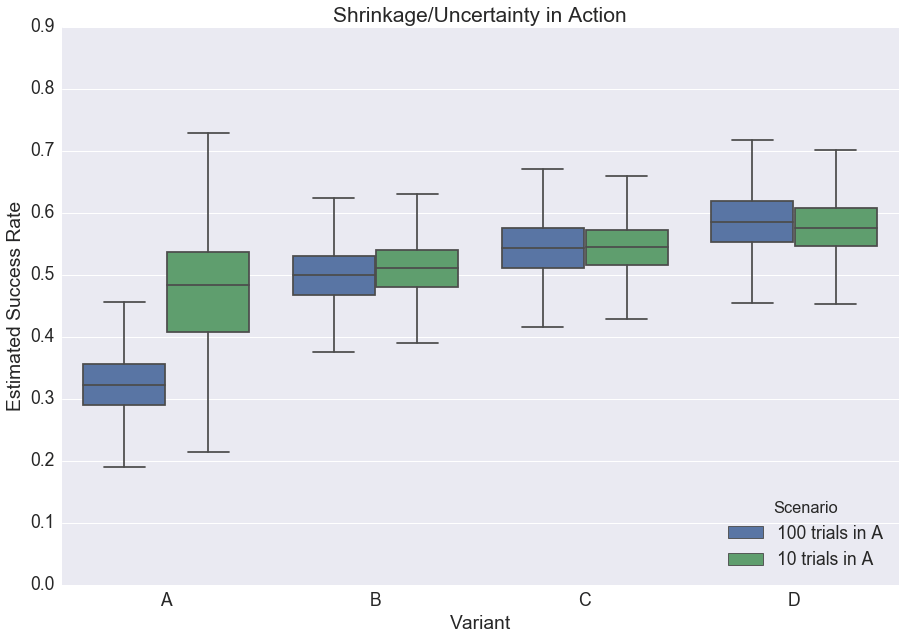
To see shrinkage in action (Adult Audiences Only), consider the following scenarios:

• In the first, there are four variants, and each has 100 trials. The observed success rates for A, B, C, and D are 30%, 50%, 55%, and 60%.
• In the second, everything is the same as the first, but variant A now has 10 trials instead of 100.

Fitting the aforementioned Beta-Binomial model — once for Scenario (A) and once for Scenario (B) — you end up with very different posterior probability distributions for variant A:

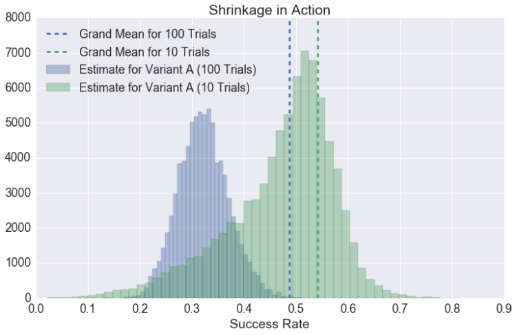
With 100 trials, our estimate for A’s success rate is pulled only slightly toward the grand rate, represented here by the blue dashed line (note that the blue posterior predictive distribution is centered at slightly above 0.3). Conversely, with only 10 trials, our mean estimate for the success rate of A is basically the same as the grand success rate. In other words, we’ve shrunk away virtually all of the A-specific information in our test.

After all, there’s only so much you can learn after 10 trials. Sorry, Product Managers.

Another way to visualize this phenomenon is in the boxplot below; notice how the success rates for all the variants change from one scenario to the next**:

Now, contrast all this with the classic approach. There, our point estimate for A’s success rate would simply be the point estimate we observed; however, we would deal with the uncertainty of comparing this rate to that of B, C, and D by penalizing the associated p-value, i.e., by requiring it to be smaller than the usual 0.05 “for significance.”

Granted: it’s not that this approach wouldn’t work. It would protect you from inflating your Type I Error, plus there are more sophisticated methods than the humble Bonferroni that won’t sap your test of its power. I merely prefer the approach that allows me to more directly model the problem at hand; that allows me to make straightforward probabilistic claims; that puts me right into modeling mode, not “consumer of various separate-but-somehow-interrelated tests” mode, which reminds me of the nightmarish way universities continue to teach statistics.

(Not to mention, p-values are silly enough without ladling on additional overhead.)

Now Let’s Get Multilevel

---

Of course, even an experiment with four variants isn’t terribly complicated. Often, however, we’re interested not only in how an experiment fares overall, but how it impacts different groups of people.

For example, say you wanted to implement a new feature on your website, and for God knows what reason, you only have users from Canada and China. Indeed, your whole company is structured around two main teams — the China Team and the Canada Team — making every experiment politically contentious, as executives from each try to one-up each other by trumpeting ever-larger, ever-faker wins.***

Consequently, every new feature necessitates an experimental design wherein you look at the impact on Canadian and Chinese users separately: a classic multiple testing problem.

This is where a multilevel model comes in. Since there are many excellent resources for a formal discussion (e.g., this one), I will again err on the side of intuition.

Consider a standard regression model, y = Treatment*x + Control.

In this scenario, you could fit two such regressions — one for Canada and one for China — but then, of course, your p-values get silly. Moreover, this strategy isn’t scalable: what happens when your VC forces your company to create its Cameroon, Cambodia, and Cayman Islands Teams? Are you really going to run separate regressions forever? That might necessitate a for loop, and we’re not software engineers!

(Note: I’m being dramatic.)

Alternatively, you could pool all the data together and fit a single such regression, thereby determining the experimental lift for your site as a whole. However, this is even more impossible: getting upper management to agree is a problem not even statistics can solve (and indeed, it usually just make things worse).

Thankfully, there’s an approach that balances the two extremes, and it’s called multilevel modeling. (Specifically, varying-intercept, varying-slope multilevel models.)

Multilevel modeling strikes a balance between the “separate” and “pooled” regression cases, and — like our simple model in the first section — relies on shrinkage to do our error correction for us. In this case, the shrinkage works not by assuming that each success rate comes from a common Beta distribution, but by assuming that the intercepts for the “China” and “Canada” regressions come from a common Gaussian distribution. Likewise for the China- and Canada-specific treatment effects, which come from a common Gaussian as well.

In other words: two regressions, but with a distributional link between the intercept terms and another distributional link between the slope terms. (Indeed, the reason the model we’re implementing is called “varying-intercept, varying-slope” is because we could have chosen to have only a single intercept or a single slope, but in this case, we want the flexibility that comes from varying both.)

If this sounds complicated, it’s because I’m a terrible explainer, so don’t get too down on yourself and Don’t Panic! As we’ll see, writing this up in PyMC3 is a pain-free process.

Do It PyMC3-Style

---

At long last, we get to the code.

• First, we import:

import numpy as np
import pandas as pd
from sklearn import preprocessing

import pymc3 as pm
import theano.tensor as T

• Next, we make a data frame consisting of our experimental data. We have one column for country (populated by a string equal to either “Canada” or “China”); one column for whether someone was in the treatment group (populated by a 0 or a 1); and one column for whether someone paid or not (populated by a 0 or a 1).

def make_dataframe(n, s):
    df = pd.DataFrame({
        'success': [0] * (n * 4),
        'country': ['Canada'] * (2 * n) + ['China'] * (2 * n),
        'treated': [0] * n + [1] * n + [0] * n + [1] * n
    })

    for i, successes in zip([n, n*2, n*3, n*4], s):
        df.loc[i - n:i - n + successes - 1, 'success'] = 1

    return df

# n, ss = 200, [60, 100, 110, 120]
n, ss = 100, [30, 50, 55, 60]

df = make_dataframe(n, ss)

• The Canada and China control groups have success rates of 30% and 55%, and the Canada and China treatment groups have success rates of 50% and 60% (i.e., conversion increased by 20 percentage points in Canada and 5 percentage points in China — please convert these to log odds if you’re a stickler). Again, we have 100 observations from each variant (presumably, Chinese and Canadian markets are equally large for us, and we ran a 50/50 test).

• To summarize it pandas-style:

df.groupby(['country', 'treated']).mean()

		success
country	treated
Canada	0	0.30
	1	0.50
China	0	0.55
	1	0.60

• For reasons I’ll get into below, we’ll need a handy way to refer to which row in our data frame is associated with which country. The LabelEncoder class from scikit-learn makes this easy-peasy:

le = preprocessing.LabelEncoder()
country_idx = le.fit_transform(df['country'])
n_countries = len(set(country_idx))

• Now, we can finally invoke the almighty PyMC (referred to as “pm” below; also, please note the comments, which we tackle post-code):

with pm.Model() as multilevel_model:

    # Hyperiors for intercept (Comment 1)
    mu_a = pm.StudentT('mu_a', nu=3, mu=0., sd=1.0)
    sigma_a = pm.HalfNormal('sigma_a', sd=1.0)

    # Hyperpriors for slope
    mu_b = pm.StudentT('mu_b', nu=3, mu=0., sd=1.0)
    sigma_b = pm.HalfNormal('sigma_b', sd=1.0)

    # Model the intercept (Comment 2)
    a = pm.Normal('a', mu=mu_a, sd=sigma_a, shape=n_countries)

    # Model the slope
    b = pm.Normal('b', mu=mu_b, sd=sigma_b, shape=n_countries)

    # Make things grok-able (Comment 3)
    a_inv = pm.Deterministic('a_inv',
                             T.exp(a)/(1 + T.exp(a)))
    fin = pm.Deterministic('fin',
                           T.exp(a + b)/(1 + T.exp(a + b)))

    # Calculate predictions given values
    # for intercept and slope (Comment 4)
    yhat = pm.invlogit(a[country_idx] +
                       b[country_idx] * df.treated.values)

    # Make predictions fit reality
    y = pm.Binomial('y', n=np.ones(df.shape[0]), p=yhat,
                    observed=df.success.values)

 

Now let’s tackle the comments:

• Comments 1-2: As I mentioned, multilevel modeling “works” by allowing you to run two pseudo-separate regressions — one for China and one for Canada — but by punishing this allowance by connecting their intercepts and slopes through common Normal distributions. To parameterize these Normal distributions, in (1) I define a pair of Student-T’s and a pair of Half-Normals, which serve as the mu and scale of the intercept/slope terms we define in (2).
  • I want to avoid a lengthy discussion as to “why these priors,” but I would note: the Half-Normal distribution is a conservative prior in that it leads to more shrinkage/partial pooling versus some other commonly-used priors****. The Stan devs have put together a phenomenal resource on selecting priors, so you can go there for more. The upshot is that the distributional assumptions of multilevel modeling work best with a large number of higher-level groups, but here, we only have two. As such, we need to be especially wary — hence the conservative Half-Normal prior. (Returning to the Lasso analogy, we’re applying more regularization here versus what we’d get with an uninformative prior, which would effectively turn this into a no-pooling regression.)
• Note that when we do parameterize the Normal for a and the Normal for b, we’re passing in a “shape” argument. This is what lets PyMC know that we’ll be taking multiple draws (i.e., China/Canada-specific slopes and intercepts) from these distributions.

• Comment 3: To keep this tutorial light, I thought I would take the inverse logit of our intercept/slope terms so that we can connect our results back to our humble data frame above. IRL, you can continue to report log-odds all you want, tiger. Note that I use the theano.tensor version of the exponent function here — this keeps PyMC3 happy since, of course, it uses theano.

• Comment 4: Here, you see what looks like a standard logistic regression formula, but with an M. Night Shyamalan-twist. Notice that we multiply the “treated” column not by b, but by b indexed to a particular country. This lets PyMC know which version of b to use — Canada-b or China-b. (Likewise for the intercept term.) (This isn’t immediately intuitive in code form, so allow me to explain: when PyMC sees the array df.treated.values, I imagine that it knows to turn the “b” term into an array of the same length. At each position in this new array, PyMC must insert either Canada-b or China-b, and the “country_idx” array is how it decides.)

• Now that we’ve built our model, we MCMC!

with multilevel_model:
    mm_trace = pm.sample(2000)

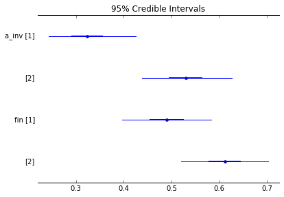
• After that’s done, we can ask our posterior probability distribution all of the scandalous, sordid, and shameful questions we’d like — no p-values or corrections required. For example, can we see a plot of all the success rates and their error bars?

pm.forestplot(mm_trace, varnames=['a_inv', 'fin'])

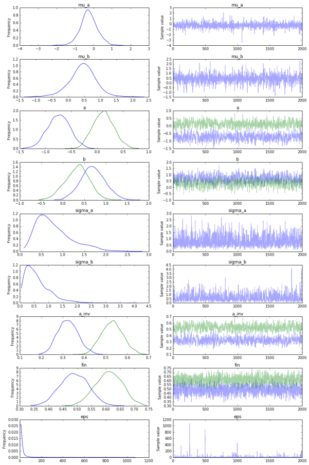
• Similarly, can we get an amazing plot that gives us a high-level summary of all the posterior distributions in our model (and how well MCMC managed to converge)?

pm.traceplot(mm_trace)

• Finally, how confident are we that the treatment boosted conversion in China?

# probability treatment better than success for China
np.mean(mm_trace.get_values('a_inv')[:, 1] <=
        mm_trace.get_values('fin')[:, 1])

• Answer: 87.3%

“Hmmm — bummer,” the Head of Team Canada might say, “because we think there’s a 99.75% chance the test improved things on our end.”

And hey — just like that, you earned that dude a promotion. Thank you, multilevel modeling!

(Code for this example available here.)

Too-Long-To-Be-An-Appendix Appendix (or: Let’s Get Unnecessarily Deep)

---

*Seriously, though, you never want to be the guy talking stats when everybody else wants to talk TayTay v. Kim K. (This and other corporate life lessons will be available in a forthcoming seminar.)

*^This didn’t really happen. I just needed a premise.

**The takeaway for our boxplot is largely the same as it is for our histogram, but with an added wrinkle: note that in our “100 Trials” scenario, our B, C, and D variants all have wider error bars than their counterparts from the “10 Trial” scenario.

This seems unintuitive, but upon inspection is unsurprising. When A has only 10 trials, the model can shrug and say, “Eh, I wouldn’t take this too seriously. Carry on, guys.” When A has 100 trials, the model can’t ignore the difference, and must reconcile A’s success rate with the very different success rates of B, C, and D — all of which presumably come from the same distribution.

It accomplishes this by widening all of the other error bars.

***I will admit: I had an ulterior motive for choosing such an extreme example. In much of the multilevel modeling literature, you will encounter a statement like this:

“Multilevel modeling only makes sense if you’re grouping by a thing that is a ‘random sample’ from some supergroup, e.g., Atlanta, Portland, Oklahoma City, Providence as representatives of the ‘US cities supergroup,’ a bunch of public school teachers as representatives of the ‘public school teacher supergroup,’ etc.

“The moment you group by something you’ve chosen for/care about specifically, it must be handled as a ‘fixed effect’ (i.e., the needlessly fancy — and probably confusing — name for a regression coefficient fit using least squares).”

For a long time, this confused the hell out of me, as it seemed to be an extreme case of the tail wagging the dog, statistical assumptions-wise. (There’s a meta point to be made here about the discipline of statistics shooting itself in the foot over and over and over again by passing on folk wisdom to people just trying to do their best and learn things, but I digress…).

In any case, I deliberately chose the literal opposite case — a company which only ever cares about two markets — to make a characteristically dramatic point. The idea isn’t whether you do or do not have groups from a larger supergroup; it’s whether you do or do not want to employ partial pooling.***(Part 2)

***(Part 2) That said, one question that did come up in my research was the number of “higher-level groups” (i.e., countries) necessary for multilevel modeling. There seems to be disagreement here, but it also seems like if you use a Bayesian approach with conservative priors (as we did here), things are okay. Plus, as Andrew Gelman says in that link, choosing not to use a multilevel model is itself a bold assumption.

Of course, if you do only have two groups, a standard regression would be totally simple given that you’d be interested in only a couple of comparisons, e.g., (1) China Treatment v. China Control and (2) Canada Treatment v. Canada Control. Obviously, multiple testing wouldn’t be much of a problem here. (I used two groups for coding convenience more than anything else, and to make this example maximally grok-able. IRL, always solve your problem using the technique that suits its best. The power of multilevel modeling really begins to make itself known when you have many, many groups that you must model and understand individually [In my domain, many, many online courses, for example].)

(For more discussion on this, check out pages 275-276 of Gelman & Hill 2007.)

****If the discussion of choosing priors makes you nervous, don’t let it! Although some folks use the notion of priors to cast aspersions on Bayesian modeling, I find it refreshing. You get to see — in code! — my priors. You get to argue with me — and even build your own model — if you disagree. If we start with different priors but end up with similar results, we can still be friends and report our results together. If we start with different (reasonable) priors and end up with very different results, then it’s a strong signal we need to collect more data.

(I should note, even if we did have many more groups than two, e.g., 20+, I would still use conservative priors as a meta-correction for all the natural incentives that skew one towards finding “real” effects where they don’t actually exist, particularly in observational, political, or small effect size contexts; see also: replication crisis, but that’s a blog post for another time…)