Dan Saber

Warning: This is a love story between a man and his Python module

As I mentioned previously, one of the most powerful concepts I’ve really learned at Zipfian has been Bayesian inference using PyMC. PyMC is currently my favorite library of any kind in any language. I dramatically italicized “learned” because I had been taught Bayesian inference in college; however, the lecture usually ended with something along the lines of, “But this gets really mathematically complicated and intense so screw it.”

In fairness, they were always at least partially right. Bayesian inference can be very mathematically complicated and intense; however, PyMC abstracts that away from you. So long as you have a coherent mental model of the problem at hand, you can apply Bayesian methods to anything (although I would note: It is worth learning the math that underlies all of this).

So as you can tell, I really, really like PyMC. 

(Indeed, this poignant romance was originally going to be the first ever blog post nominated for an Academy Award, but Her came out and mined much of the same emotional territory. I gracefully stepped aside and let Spike Jonze, Joaquin Phoenix and Scarlett Johansson have their fifteen minutes…

…The Academy Awards are pure politics anyway.)

What we’ll cover

In this example, I’m going to demonstrate how you can use Bayesian inference with PyMC to estimate the parameters of a linear regression problem. I think this example is particularly well-suited for a tutorial because: (A) A lot of people learn linear regression in college, so hopefully you’ll readily understand the model necessary to solve the problem; and (B) The numbers that emerge are readily meaningful and interpretable.

I’m first going to cover the Single Variable case, and then I’ll share my model for the Multivariable case. 

Single Variable Bayesian Regression

For this example, we’re going to try to model the mpg of a car as a function of the car’s weight, i.e., mpg = b0 + b1 * weight + error. In the example below, the Data Frame I’m using is named “float_df,” and the column names are self-explanatory. 

As usual, we begin by importing our friends: For this exercise, we’ll need pymc, numpy, pandas, and matplotlib.pyplot, which I refer to below as pymc, np, pd and plt, respectively. 

Next, we’ll need to set up the model. I explain what I’m doing in the included comments, but I will come back to the most important parts below. 

# NOTE: the linear regression model we're trying to solve for is
# given by:
# y = b0 + b1(x) + error
# where b0 is the intercept term, b1 is the slope, and error is
# the error

# model the intercept/slope terms of our model as
# normal random variables with comically large variances
b0 = pymc.Normal('b0', 0, 0.0003)
b1 = pymc.Normal('b1', 0, 0.0003)

# model our error term as a uniform random variable
err = pymc.Uniform('err', 0, 500)

# "model" the observed x values as a normal random variable
# in reality, because x is observed, it doesn't actually matter
# how we choose to model x -- PyMC isn't going to change x's values
x_weight = pymc.Normal('weight' 0, 1, value=np.array(float_df['weight']), observed=True)

# this is the heart of our model: given our b0, b1 and our x observations, we want
# to predict y
@pymc.deterministic
def pred(b0=b0, b1=b1, x=x_weight):
return b0 + b1*x

# "model" the observed y values: again, I reiterate that PyMC treats y as
# evidence -- as fixed; it's going to use this as evidence in updating our belief
# about the "unobserved" parameters (b0, b1, and err), which are the
# things we're interested in inferring after all
y = pymc.Normal('y', pred, err, value=np.array(float_df['mpg']), observed=True)

# put everything we've modeled into a PyMC model
model = pymc.Model([pred, b0, b1, y, err, x_weight])

The aforementioned core concepts:

• Everything in PyMC is a random variable, but some are more random than others. What do I mean? Objects in PyMC are either “Stochastic,” as is the case for our err and beta terms, or “Deterministic,” as in the case of our predicted y values. Deterministic may not have been the most accurate expression because deterministic variables are themselves random by way of their inputs. In this case, deterministic simply means that given the values we pass into our deterministic function, it’s possible to know with certainty what value that function will return. Contrast this with our err term: We’re given its inputs — they’re 0 and 500 — but this says nothing about what err actually is other than that it’s between 0 and 500. 

• The other critical notion is “observed” versus “unobserved.” In the Bayesian world, our distribution parameters are random variables, and our observations are fixed: They’re the mechanism by which we can update the probability distribution of our parameters. For this reason, it is somewhat important that we let our model know about them. In our case, we have two sets of observations, the weight of our cars and their associated mpg number. The observed mpg data makes its way into our model via the “y” normal random variable, and the observed weight data makes its way into our model via the “x_weight” normal random variable.

• I mentioned it in the comments of my code and the paragraph above, but I’ll reiterate it here: our observed x and y values are fixed*. This view is in direct contrast to the Frequentist approach, in which the data are random variables, the parameters are fixed, and we’re trying to determine how likely it is that we would see the data given a particular view of the world (i.e., a particular view of our parameters).

• Phrasing it this way, it’s clear that the Bayesian approach is the more intuitive one. We’ve already observed the data: Now how does this data update our belief about the underlying parameters? This conceptual elegance is why Bayesians like to say obnoxious-but-accurate things like, “You’re born a Bayesian. You need to be taught to be a Frequentist.”

• We’ve given the elements in our model “priors,” an important notion in Bayesian statistics. For example, by modeling our error term as a Uniform random variable between 0 and 500, we’re essentially saying, “Between 0 and 500, I have absolutely no idea where the true error lies — all values are equally likely. However, outside of that range, I am gravely certain that we will not find the value of our error.” Similarly, by modeling our betas as Normal variables with mean 0 and an immense variance, we’re saying, “I’m essentially assuming there’s no relationship between X and Y, but don’t quote me on that because who knows.” These priors are what you would call “uninformative” — as in, we’re mostly just going to let the data inform the majority of our worldview.

Whew. Get all that? I didn’t the first time around, so if you’re still in need of some help I, would check out PyMC’s official tutorial. 

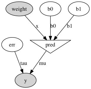
An exceedingly helpful way of visualizing our model and ensuring that we set everything up exactly as we intended is by using the “graph” module. I’ve included the code and the resultant model below:

import pymc.graph
graph = pymc.graph.graph(model)
graph.write_png('univariate.png')

We get that for free — immensely cool.

Now that we’ve done the legwork of setting up our model, PyMC can work its magic:

# prepare for MCMC
mcmc = pymc.MCMC(model)

# sample from our posterior distribution 50,000 times, but
# throw the first 20,000 samples out to ensure that we're only
# sampling from our steady-state posterior distribution
mcmc.sample(50000, 20000)

By invoking pymc.MCMC() and passing in our model, we can sample values from the steady-state posterior distribution of our model thousands and thousands of times. The notion of “steady-state” is why we pass 20000 as the second argument to the sample method: We don’t want to record samples before MCMC has converged on a solution, so we throw out the first 20,000. This creates a probability distribution for the various non-observed inputs of our model. To get a more in-depth idea of how MCMC works, I found this lecture amazingly helpful. UPDATE: One of my classmates, Jonny Lee, also wrote a great post specific to this topic here. 

After sampling our posterior distribution, which again, was developed as a “combination” of our prior beliefs and our observed data, we can do things like this:

print np.mean(mcmc.trace('b1')[:])
plt.hist(mcmc.trace('b1')[:], bins=50)

This is the probability distribution of our slope term: It allows us to say incredible things like, “A one-unit increase in the weight of a car is associated with a decrease in its mpg, and we’re virtually certain that the magnitude of this decrease is between -0.0085 and -0.007 units.”

The Multivariable Case

The multivariable case isn’t very different from the above. There’s simply the added concept of a PyMC “Container,” which binds similar random variables together in a coherent way (important when you have multiple betas to solve for).

The code for setting up this case is below:

def linear_setup(df, ind_cols, dep_col):
'''
Inputs: pandas Data Frame, list of strings for the independent variables,
single string for the dependent variable
Output: PyMC Model
'''

# model our intercept and error term as above
b0 = pymc.Normal('b0', 0, 0.0001)
err = pymc.Uniform('err', 0, 500)

# initialize a NumPy array to hold our betas
# and our observed x values
b = np.empty(len(ind_cols), dtype=object)
x = np.empty(len(ind_cols), dtype=object)

# loop through b, and make our ith beta
# a normal random variable, as in the single variable case
for i in range(len(b)):
b[i] = pymc.Normal('b' + str(i + 1), 0, 0.0001)

# loop through x, and inform our model about the observed
# x values that correspond to the ith position
for i, col in enumerate(ind_cols):
x[i] = pymc.Normal('b' + str(i + 1), 0, 1, value=np.array(df[col]), observed=True)

# as above, but use .dot() for 2D array (i.e., matrix) multiplication
@pymc.deterministic
def y_pred(b0=b0, b=b, x=x):
return b0 + b.dot(x)

# finally, "model" our observed y values as above
y = pymc.Normal('y', y_pred, err, value=np.array(df[dep_col]), observed=True)

return pymc.Model([b0, pymc.Container(b), err, pymc.Container(x), y, y_pred])

And here’s an example (for the example, our independent variables are “weight” and “acceleration,” and our dependent variable is still “mpg”).

test_model = linear_setup(float_df, ['weight', 'acceleration'], 'mpg')
mcmc = pymc.MCMC(test_model)
mcmc.sample(100000, 20000)

Now that we’ve sampled our posterior, we can again plot the marginal probability distributions of our beta terms:

multifig, multiax = plt.subplots(2, 1, figsize=(10, 10))
b_nought = mcmc.trace('b0')[:]
b_weight = mcmc.trace('b1')[:]
b_accelerate = mcmc.trace('b2')[:]

multiax[0].hist(b_weight)
multiax[0].set_title('Weight Coefficient Probability Distribution')
multiax[1].hist(b_accelerate)
multiax[1].set_title('Acceleration Coefficient Probability Distribution')

Finally, to tie everything together and solidify our mental model, I include the means of the histograms I plotted above along with the mean of our intercept term. I also provide the results of using OLS. You’ll find that the two are quite similar…

Bayesian

print 'Intercept: ' + str(np.mean(b_nought))
print 'Weight Coefficient: ' + str(np.mean(b_weight))
print 'Acceleration Coefficient: ' + str(np.mean(b_accelerate))

# prints
# Intercept: 41.0051165145
# Weight Coefficient: -0.00729068321556
# Acceleration Coefficient: 0.267134957533

OLS

coef    std err          t      P>|t|      [95.0% Conf. Int.]
------------------------------------------------------------------------------
const         41.0953      1.868     21.999      0.000        37.423    44.768
x1            -0.0073      0.000    -25.966      0.000        -0.008    -0.007
x2             0.2617      0.086      3.026      0.003         0.092     0.432

And there you have it. A lot of work whose results we could have duplicated in a single line of code using the statsmodels package, but doesn’t this make you feel a lot more accomplished?

Wonderful!